


标签传播算法(Label Propagation)及Python实现
众所周知,机器学习可以大体分为三大类:监督学习、非监督学习和半监督学习。监督学习可以认为是我们有非常多的labeled标注数据来train一个模型,期待这个模型能学习到数据的分布,以期对未来没有见到的样本做预测。那这个性能的源头--训练数据,就显得非常感觉。你必须有足够的训练数据,以覆盖真正现实数据中的样本分布才可以,这样学习到的模型才有意义。那非监督学习就是没有任何的labeled数据,就是平时所说的聚类了,利用他们本身的数据分布,给他们划分类别。而半监督学习,顾名思义就是处于两者之间的,只有少量的labeled数据,我们试图从这少量的labeled数据和大量的unlabeled数据中学习到有用的信息。
一、半监督学习
半监督学习(Semi-supervised learning)发挥作用的场合是:你的数据有一些有label,一些没有。而且一般是绝大部分都没有,只有少许几个有label。半监督学习算法会充分的利用unlabeled数据来捕捉我们整个数据的潜在分布。它基于三大假设:
1)Smoothness平滑假设:相似的数据具有相同的label。
2)Cluster聚类假设:处于同一个聚类下的数据具有相同label。
3)Manifold流形假设:处于同一流形结构下的数据具有相同label。
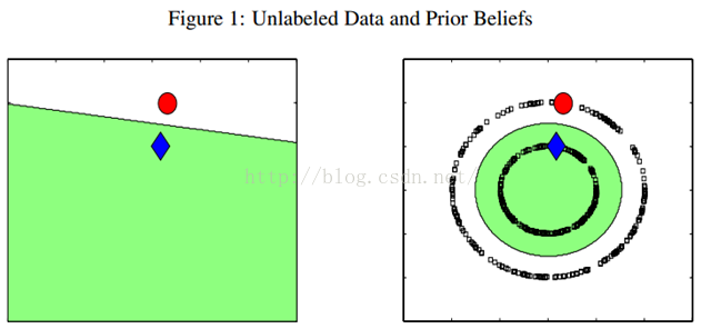
例如下图,只有两个labeled数据,如果直接用他们来训练一个分类器,例如LR或者SVM,那么学出来的分类面就是左图那样的。如果现实中,这个数据是右图那边分布的话,猪都看得出来,左图训练的这个分类器烂的一塌糊涂、惨不忍睹。因为我们的labeled训练数据太少了,都没办法覆盖我们未来可能遇到的情况。但是,如果右图那样,把大量的unlabeled数据(黑色的)都考虑进来,有个全局观念,牛逼的算法会发现,哎哟,原来是两个圈圈(分别处于两个圆形的流形之上)!那算法就很聪明,把大圈的数据都归类为红色类别,把内圈的数据都归类为蓝色类别。因为,实践中,labeled数据是昂贵,很难获得的,但unlabeled数据就不是了,写个脚本在网上爬就可以了,因此如果能充分利用大量的unlabeled数据来辅助提升我们的模型学习,这个价值就非常大。
半监督学习算法有很多,下面我们介绍最简单的标签传播算法(label propagation),最喜欢简单了,哈哈。
二、标签传播算法
标签传播算法(label propagation)的核心思想非常简单:相似的数据应该具有相同的label。LP算法包括两大步骤:1)构造相似矩阵;2)勇敢的传播吧。
2.1、相似矩阵构建
LP算法是基于Graph的,因此我们需要先构建一个图。我们为所有的数据构建一个图,图的节点就是一个数据点,包含labeled和unlabeled的数据。节点i和节点j的边表示他们的相似度。这个图的构建方法有很多,这里我们假设这个图是全连接的,节点i和节点j的边权重为:
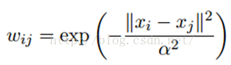
这里,α是超参。
还有个非常常用的图构建方法是knn图,也就是只保留每个节点的k近邻权重,其他的为0,也就是不存在边,因此是稀疏的相似矩阵。
2.2、LP算法
标签传播算法非常简单:通过节点之间的边传播label。边的权重越大,表示两个节点越相似,那么label越容易传播过去。我们定义一个NxN的概率转移矩阵P:
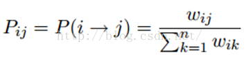
Pij表示从节点i转移到节点j的概率。假设有C个类和L个labeled样本,我们定义一个LxC的label矩阵YL,第i行表示第i个样本的标签指示向量,即如果第i个样本的类别是j,那么该行的第j个元素为1,其他为0。同样,我们也给U个unlabeled样本一个UxC的label矩阵YU。把他们合并,我们得到一个NxC的soft label矩阵F=[YL;YU]。soft label的意思是,我们保留样本i属于每个类别的概率,而不是互斥性的,这个样本以概率1只属于一个类。当然了,最后确定这个样本i的类别的时候,是取max也就是概率最大的那个类作为它的类别的。那F里面有个YU,它一开始是不知道的,那最开始的值是多少?无所谓,随便设置一个值就可以了。
千呼万唤始出来,简单的LP算法如下:
1)执行传播:F=PF
2)重置F中labeled样本的标签:FL=YL
3)重复步骤1)和2)直到F收敛。
步骤1)就是将矩阵P和矩阵F相乘,这一步,每个节点都将自己的label以P确定的概率传播给其他节点。如果两个节点越相似(在欧式空间中距离越近),那么对方的label就越容易被自己的label赋予,就是更容易拉帮结派。步骤2)非常关键,因为labeled数据的label是事先确定的,它不能被带跑,所以每次传播完,它都得回归它本来的label。随着labeled数据不断的将自己的label传播出去,最后的类边界会穿越高密度区域,而停留在低密度的间隔中。相当于每个不同类别的labeled样本划分了势力范围。
2.3、变身的LP算法
我们知道,我们每次迭代都是计算一个soft label矩阵F=[YL;YU],但是YL是已知的,计算它没有什么用,在步骤2)的时候,还得把它弄回来。我们关心的只是YU,那我们能不能只计算YU呢?Yes。我们将矩阵P做以下划分:
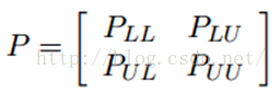
这时候,我们的算法就一个运算:
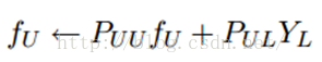
迭代上面这个步骤直到收敛就ok了,是不是很cool。可以看到FU不但取决于labeled数据的标签及其转移概率,还取决了unlabeled数据的当前label和转移概率。因此LP算法能额外运用unlabeled数据的分布特点。
这个算法的收敛性也非常容易证明,具体见参考文献[1]。实际上,它是可以收敛到一个凸解的:
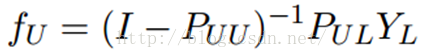
所以我们也可以直接这样求解,以获得最终的YU。但是在实际的应用过程中,由于矩阵求逆需要O(n3)的复杂度,所以如果unlabeled数据非常多,那么I – PUU矩阵的求逆将会非常耗时,因此这时候一般选择迭代算法来实现。
三、LP算法的Python实现
Python环境的搭建就不啰嗦了,可以参考前面的博客。需要额外依赖的库是经典的numpy和matplotlib。代码中包含了两种图的构建方法:RBF和KNN指定。同时,自己生成了两个toy数据库:两条长形形状和两个圈圈的数据。第四部分我们用大点的数据库来做实验,先简单的可视化验证代码的正确性,再前线。
算法代码:
#***************************************************************************
#*
#* Description: label propagation
#* Author: Zou Xiaoyi (zouxy09@qq.com)
#* Date:   2015-10-15
#* HomePage: http://blog.csdn.net/zouxy09
#*
#**************************************************************************

import time
import numpy as np

# return k neighbors index
def navie_knn(dataSet, query, k):
    numSamples = dataSet.shape[0]

    ## step 1: calculate Euclidean distance
    diff = np.tile(query, (numSamples, 1)) - dataSet
    squaredDiff = diff ** 2
    squaredDist = np.sum(squaredDiff, axis = 1) # sum is performed by row

    ## step 2: sort the distance
    sortedDistIndices = np.argsort(squaredDist)
    if k > len(sortedDistIndices):
        k = len(sortedDistIndices)

    return sortedDistIndices[0:k]


# build a big graph (normalized weight matrix)
def buildGraph(MatX, kernel_type, rbf_sigma = None, knn_num_neighbors = None):
    num_samples = MatX.shape[0]
    affinity_matrix = np.zeros((num_samples, num_samples), np.float32)
    if kernel_type == 'rbf':
        if rbf_sigma == None:
            raise ValueError('You should input a sigma of rbf kernel!')
        for i in xrange(num_samples):
            row_sum = 0.0
            for j in xrange(num_samples):
                diff = MatX[i, :] - MatX[j, :]
                affinity_matrix[i][j] = np.exp(sum(diff**2) / (-2.0 * rbf_sigma**2))
                row_sum += affinity_matrix[i][j]
            affinity_matrix[i][:] /= row_sum
    elif kernel_type == 'knn':
        if knn_num_neighbors == None:
            raise ValueError('You should input a k of knn kernel!')
        for i in xrange(num_samples):
            k_neighbors = navie_knn(MatX, MatX[i, :], knn_num_neighbors)
            affinity_matrix[i][k_neighbors] = 1.0 / knn_num_neighbors
    else:
        raise NameError('Not support kernel type! You can use knn or rbf!')

    return affinity_matrix


# label propagation
def labelPropagation(Mat_Label, Mat_Unlabel, labels, kernel_type = 'rbf', rbf_sigma = 1.5, \
                    knn_num_neighbors = 10, max_iter = 500, tol = 1e-3):
    # initialize
    num_label_samples = Mat_Label.shape[0]
    num_unlabel_samples = Mat_Unlabel.shape[0]
    num_samples = num_label_samples + num_unlabel_samples
    labels_list = np.unique(labels)
    num_classes = len(labels_list)

    MatX = np.vstack((Mat_Label, Mat_Unlabel))
    clamp_data_label = np.zeros((num_label_samples, num_classes), np.float32)
    for i in xrange(num_label_samples):
        clamp_data_label[i][labels[i]] = 1.0

    label_function = np.zeros((num_samples, num_classes), np.float32)
    label_function[0 : num_label_samples] = clamp_data_label
    label_function[num_label_samples : num_samples] = -1

    # graph construction
    affinity_matrix = buildGraph(MatX, kernel_type, rbf_sigma, knn_num_neighbors)

    # start to propagation
    iter = 0; pre_label_function = np.zeros((num_samples, num_classes), np.float32)
    changed = np.abs(pre_label_function - label_function).sum()
    while iter < max_iter and changed > tol:
        if iter % 1 == 0:
            print "---> Iteration %d/%d, changed: %f" % (iter, max_iter, changed)
        pre_label_function = label_function
        iter += 1

        # propagation
        label_function = np.dot(affinity_matrix, label_function)

        # clamp
        label_function[0 : num_label_samples] = clamp_data_label

        # check converge
        changed = np.abs(pre_label_function - label_function).sum()

    # get terminate label of unlabeled data
    unlabel_data_labels = np.zeros(num_unlabel_samples)
    for i in xrange(num_unlabel_samples):
        unlabel_data_labels[i] = np.argmax(label_function[i+num_label_samples])

    return unlabel_data_labels
测试代码:
#***************************************************************************
#*
#* Description: label propagation
#* Author: Zou Xiaoyi (zouxy09@qq.com)
#* Date:   2015-10-15
#* HomePage: http://blog.csdn.net/zouxy09
#*
#**************************************************************************

import time
import math
import numpy as np
from label_propagation import labelPropagation

# show
def show(Mat_Label, labels, Mat_Unlabel, unlabel_data_labels):
    import matplotlib.pyplot as plt

    for i in range(Mat_Label.shape[0]):
        if int(labels[i]) == 0:
            plt.plot(Mat_Label[i, 0], Mat_Label[i, 1], 'Dr')
        elif int(labels[i]) == 1:
            plt.plot(Mat_Label[i, 0], Mat_Label[i, 1], 'Db')
        else:
            plt.plot(Mat_Label[i, 0], Mat_Label[i, 1], 'Dy')

    for i in range(Mat_Unlabel.shape[0]):
        if int(unlabel_data_labels[i]) == 0:
            plt.plot(Mat_Unlabel[i, 0], Mat_Unlabel[i, 1], 'or')
        elif int(unlabel_data_labels[i]) == 1:
            plt.plot(Mat_Unlabel[i, 0], Mat_Unlabel[i, 1], 'ob')
        else:
            plt.plot(Mat_Unlabel[i, 0], Mat_Unlabel[i, 1], 'oy')

    plt.xlabel('X1'); plt.ylabel('X2')
    plt.xlim(0.0, 12.)
    plt.ylim(0.0, 12.)
    plt.show()


def loadCircleData(num_data):
    center = np.array([5.0, 5.0])
    radiu_inner = 2
    radiu_outer = 4
    num_inner = num_data / 3
    num_outer = num_data - num_inner

    data = []
    theta = 0.0
    for i in range(num_inner):
        pho = (theta % 360) * math.pi / 180
        tmp = np.zeros(2, np.float32)
        tmp[0] = radiu_inner * math.cos(pho) + np.random.rand(1) + center[0]
        tmp[1] = radiu_inner * math.sin(pho) + np.random.rand(1) + center[1]
        data.append(tmp)
        theta += 2

    theta = 0.0
    for i in range(num_outer):
        pho = (theta % 360) * math.pi / 180
        tmp = np.zeros(2, np.float32)
        tmp[0] = radiu_outer * math.cos(pho) + np.random.rand(1) + center[0]
        tmp[1] = radiu_outer * math.sin(pho) + np.random.rand(1) + center[1]
        data.append(tmp)
        theta += 1

    Mat_Label = np.zeros((2, 2), np.float32)
    Mat_Label[0] = center + np.array([-radiu_inner + 0.5, 0])
    Mat_Label[1] = center + np.array([-radiu_outer + 0.5, 0])
    labels = [0, 1]
    Mat_Unlabel = np.vstack(data)
    return Mat_Label, labels, Mat_Unlabel


def loadBandData(num_unlabel_samples):
    #Mat_Label = np.array([[5.0, 2.], [5.0, 8.0]])
    #labels = [0, 1]
    #Mat_Unlabel = np.array([[5.1, 2.], [5.0, 8.1]])

    Mat_Label = np.array([[5.0, 2.], [5.0, 8.0]])
    labels = [0, 1]
    num_dim = Mat_Label.shape[1]
    Mat_Unlabel = np.zeros((num_unlabel_samples, num_dim), np.float32)
    Mat_Unlabel[:num_unlabel_samples/2, :] = (np.random.rand(num_unlabel_samples/2, num_dim) - 0.5) * np.array([3, 1]) + Mat_Label[0]
    Mat_Unlabel[num_unlabel_samples/2 : num_unlabel_samples, :] = (np.random.rand(num_unlabel_samples/2, num_dim) - 0.5) * np.array([3, 1]) + Mat_Label[1]
    return Mat_Label, labels, Mat_Unlabel


# main function
if __name__ == "__main__":
    num_unlabel_samples = 800
    #Mat_Label, labels, Mat_Unlabel = loadBandData(num_unlabel_samples)
    Mat_Label, labels, Mat_Unlabel = loadCircleData(num_unlabel_samples)

    ## Notice: when use 'rbf' as our kernel, the choice of hyper parameter 'sigma' is very import! It should be
    ## chose according to your dataset, specific the distance of two data points. I think it should ensure that
    ## each point has about 10 knn or w_i,j is large enough. It also influence the speed of converge. So, may be
    ## 'knn' kernel is better!
    #unlabel_data_labels = labelPropagation(Mat_Label, Mat_Unlabel, labels, kernel_type = 'rbf', rbf_sigma = 0.2)
    unlabel_data_labels = labelPropagation(Mat_Label, Mat_Unlabel, labels, kernel_type = 'knn', knn_num_neighbors = 10, max_iter = 400)
    show(Mat_Label, labels, Mat_Unlabel, unlabel_data_labels)
该注释的,代码都注释的,有看不明白的,欢迎交流。不同迭代次数时候的结果如下:
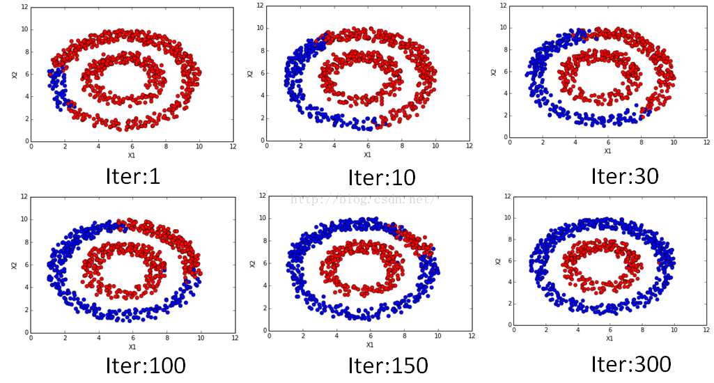
是不是很漂亮的传播过程?!在数值上也是可以看到随着迭代的进行逐渐收敛的,迭代的数值变化过程如下:
---> Iteration 0/400, changed: 1602.000000
---> Iteration 1/400, changed: 6.300182
---> Iteration 2/400, changed: 5.129996
---> Iteration 3/400, changed: 4.301994
---> Iteration 4/400, changed: 3.819295
---> Iteration 5/400, changed: 3.501743
---> Iteration 6/400, changed: 3.277122
---> Iteration 7/400, changed: 3.105952
---> Iteration 8/400, changed: 2.967030
---> Iteration 9/400, changed: 2.848606
---> Iteration 10/400, changed: 2.743997
---> Iteration 11/400, changed: 2.649270
---> Iteration 12/400, changed: 2.562057
---> Iteration 13/400, changed: 2.480885
---> Iteration 14/400, changed: 2.404774
---> Iteration 15/400, changed: 2.333075
---> Iteration 16/400, changed: 2.265301
---> Iteration 17/400, changed: 2.201107
---> Iteration 18/400, changed: 2.140209
---> Iteration 19/400, changed: 2.082354
---> Iteration 20/400, changed: 2.027376
---> Iteration 21/400, changed: 1.975071
---> Iteration 22/400, changed: 1.925286
---> Iteration 23/400, changed: 1.877894
---> Iteration 24/400, changed: 1.832743
---> Iteration 25/400, changed: 1.789721
---> Iteration 26/400, changed: 1.748706
---> Iteration 27/400, changed: 1.709593
---> Iteration 28/400, changed: 1.672284
---> Iteration 29/400, changed: 1.636668
---> Iteration 30/400, changed: 1.602668
---> Iteration 31/400, changed: 1.570200
---> Iteration 32/400, changed: 1.539179
---> Iteration 33/400, changed: 1.509530
---> Iteration 34/400, changed: 1.481182
---> Iteration 35/400, changed: 1.454066
---> Iteration 36/400, changed: 1.428120
---> Iteration 37/400, changed: 1.403283
---> Iteration 38/400, changed: 1.379502
---> Iteration 39/400, changed: 1.356734
---> Iteration 40/400, changed: 1.334906
---> Iteration 41/400, changed: 1.313983
---> Iteration 42/400, changed: 1.293921
---> Iteration 43/400, changed: 1.274681
---> Iteration 44/400, changed: 1.256214
---> Iteration 45/400, changed: 1.238491
---> Iteration 46/400, changed: 1.221474
---> Iteration 47/400, changed: 1.205126
---> Iteration 48/400, changed: 1.189417
---> Iteration 49/400, changed: 1.174316
---> Iteration 50/400, changed: 1.159804
---> Iteration 51/400, changed: 1.145844
---> Iteration 52/400, changed: 1.132414
---> Iteration 53/400, changed: 1.119490
---> Iteration 54/400, changed: 1.107032
---> Iteration 55/400, changed: 1.095054
---> Iteration 56/400, changed: 1.083513
---> Iteration 57/400, changed: 1.072397
---> Iteration 58/400, changed: 1.061671
---> Iteration 59/400, changed: 1.051324
---> Iteration 60/400, changed: 1.041363
---> Iteration 61/400, changed: 1.031742
---> Iteration 62/400, changed: 1.022459
---> Iteration 63/400, changed: 1.013494
---> Iteration 64/400, changed: 1.004836
---> Iteration 65/400, changed: 0.996484
---> Iteration 66/400, changed: 0.988407
---> Iteration 67/400, changed: 0.980592
---> Iteration 68/400, changed: 0.973045
---> Iteration 69/400, changed: 0.965744
---> Iteration 70/400, changed: 0.958682
---> Iteration 71/400, changed: 0.951848
---> Iteration 72/400, changed: 0.945227
---> Iteration 73/400, changed: 0.938820
---> Iteration 74/400, changed: 0.932608
---> Iteration 75/400, changed: 0.926590
---> Iteration 76/400, changed: 0.920765
---> Iteration 77/400, changed: 0.915107
---> Iteration 78/400, changed: 0.909628
---> Iteration 79/400, changed: 0.904309
---> Iteration 80/400, changed: 0.899143
---> Iteration 81/400, changed: 0.894122
---> Iteration 82/400, changed: 0.889259
---> Iteration 83/400, changed: 0.884530
---> Iteration 84/400, changed: 0.879933
---> Iteration 85/400, changed: 0.875464
---> Iteration 86/400, changed: 0.871121
---> Iteration 87/400, changed: 0.866888
---> Iteration 88/400, changed: 0.862773
---> Iteration 89/400, changed: 0.858783
---> Iteration 90/400, changed: 0.854879
---> Iteration 91/400, changed: 0.851084
---> Iteration 92/400, changed: 0.847382
---> Iteration 93/400, changed: 0.843779
---> Iteration 94/400, changed: 0.840274
---> Iteration 95/400, changed: 0.836842
---> Iteration 96/400, changed: 0.833501
---> Iteration 97/400, changed: 0.830240
---> Iteration 98/400, changed: 0.827051
---> Iteration 99/400, changed: 0.823950
---> Iteration 100/400, changed: 0.820906
---> Iteration 101/400, changed: 0.817946
---> Iteration 102/400, changed: 0.815053
---> Iteration 103/400, changed: 0.812217
---> Iteration 104/400, changed: 0.809437
---> Iteration 105/400, changed: 0.806724
---> Iteration 106/400, changed: 0.804076
---> Iteration 107/400, changed: 0.801480
---> Iteration 108/400, changed: 0.798937
---> Iteration 109/400, changed: 0.796448
---> Iteration 110/400, changed: 0.794008
---> Iteration 111/400, changed: 0.791612
---> Iteration 112/400, changed: 0.789282
---> Iteration 113/400, changed: 0.786984
---> Iteration 114/400, changed: 0.784728
---> Iteration 115/400, changed: 0.782516
---> Iteration 116/400, changed: 0.780355
---> Iteration 117/400, changed: 0.778216
---> Iteration 118/400, changed: 0.776139
---> Iteration 119/400, changed: 0.774087
---> Iteration 120/400, changed: 0.772072
---> Iteration 121/400, changed: 0.770085
---> Iteration 122/400, changed: 0.768146
---> Iteration 123/400, changed: 0.766232
---> Iteration 124/400, changed: 0.764356
---> Iteration 125/400, changed: 0.762504
---> Iteration 126/400, changed: 0.760685
---> Iteration 127/400, changed: 0.758889
---> Iteration 128/400, changed: 0.757135
---> Iteration 129/400, changed: 0.755406
四、LP算法MPI并行实现
这里,我们测试的是LP的变身版本。从公式,我们可以看到,第二项PULYL迭代过程并没有发生变化,所以这部分实际上从迭代开始就可以计算好,从而避免重复计算。不过,不管怎样,LP算法都要计算一个UxU的矩阵PUU和一个UxC矩阵FU的乘积。当我们的unlabeled数据非常多,而且类别也很多的时候,计算是很慢的,同时占用的内存量也非常大。另外,构造Graph需要计算两两的相似度,也是O(n2)的复杂度,当我们数据的特征维度很大的时候,这个计算量也是非常客观的。所以我们就得考虑并行处理了。而且最好是能放到集群上并行。那如何并行呢?
对算法的并行化,一般分为两种:数据并行和模型并行。
数据并行很好理解,就是将数据划分,每个节点只处理一部分数据,例如我们构造图的时候,计算每个数据的k近邻。例如我们有1000个样本和20个CPU节点,那么就平均分发,让每个CPU节点计算50个样本的k近邻,然后最后再合并大家的结果。可见这个加速比也是非常可观的。
模型并行一般发生在模型很大,无法放到单机的内存里面的时候。例如庞大的深度神经网络训练的时候,就需要把这个网络切开,然后分别求解梯度,最后有个leader的节点来收集大家的梯度,再反馈给大家去更新。当然了,其中存在更细致和高效的工程处理方法。在我们的LP算法中,也是可以做模型并行的。假如我们的类别数C很大,把类别数切开,让不同的CPU节点处理,实际上就相当于模型并行了。
那为啥不切大矩阵PUU,而是切小点的矩阵FU,因为大矩阵PUU没法独立分块,并行的一个原则是处理必须是独立的。 矩阵FU依赖的是所有的U,而把PUU切开分发到其他节点的时候,每次FU的更新都需要和其他的节点通信,这个通信的代价是很大的(实际上,很多并行系统没法达到线性的加速度的瓶颈是通信!线性加速比是,我增加了n台机器,速度就提升了n倍)。但是对类别C也就是矩阵FU切分,就不会有这个问题,因为他们的计算是独立的。只是决定样本的最终类别的时候,将所有的FU收集回来求max就可以了。
所以,在下面的代码中,是同时包含了数据并行和模型并行的雏形的。另外,还值得一提的是,我们是迭代算法,那决定什么时候迭代算法停止?除了判断收敛外,我们还可以让每迭代几步,就用测试label测试一次结果,看模型的整体训练性能如何。特别是判断训练是否过拟合的时候非常有效。因此,代码中包含了这部分内容。
好了,代码终于来了。大家可以搞点大数据库来测试,如果有MPI集群条件的话就更好了。
下面的代码依赖numpy、scipy(用其稀疏矩阵加速计算)和mpi4py。其中mpi4py需要依赖openmpi和Cpython,可以参考我之前的博客进行安装。
#***************************************************************************
#*
#* Description: label propagation
#* Author: Zou Xiaoyi (zouxy09@qq.com)
#* Date:   2015-10-15
#* HomePage: http://blog.csdn.net/zouxy09
#*
#**************************************************************************

import os, sys, time
import numpy as np
from scipy.sparse import csr_matrix, lil_matrix, eye
import operator
import cPickle as pickle
import mpi4py.MPI as MPI

#
#   Global variables for MPI
#

# instance for invoking MPI related functions
comm = MPI.COMM_WORLD
# the node rank in the whole community
comm_rank = comm.Get_rank()
# the size of the whole community, i.e., the total number of working nodes in the MPI cluster
comm_size = comm.Get_size()

# load mnist dataset
def load_MNIST():
    import gzip
    f = gzip.open("mnist.pkl.gz", "rb")
    train, val, test = pickle.load(f)
    f.close()

    Mat_Label = train[0]
    labels = train[1]
    Mat_Unlabel = test[0]
    groundtruth = test[1]
    labels_id = [0, 1, 2, 3, 4, 5, 6, 7, 8, 9]

    return Mat_Label, labels, labels_id, Mat_Unlabel, groundtruth

# return k neighbors index
def navie_knn(dataSet, query, k):
    numSamples = dataSet.shape[0]

    ## step 1: calculate Euclidean distance
    diff = np.tile(query, (numSamples, 1)) - dataSet
    squaredDiff = diff ** 2
    squaredDist = np.sum(squaredDiff, axis = 1) # sum is performed by row

    ## step 2: sort the distance
    sortedDistIndices = np.argsort(squaredDist)
    if k > len(sortedDistIndices):
        k = len(sortedDistIndices)
    return sortedDistIndices[0:k]


# build a big graph (normalized weight matrix)
# sparse U x (U + L) matrix
def buildSubGraph(Mat_Label, Mat_Unlabel, knn_num_neighbors):
    num_unlabel_samples = Mat_Unlabel.shape[0]
    data = []; indices = []; indptr = [0]
    Mat_all = np.vstack((Mat_Label, Mat_Unlabel))
    values = np.ones(knn_num_neighbors, np.float32) / knn_num_neighbors
    for i in xrange(num_unlabel_samples):
        k_neighbors = navie_knn(Mat_all, Mat_Unlabel[i, :], knn_num_neighbors)
        indptr.append(np.int32(indptr[-1]) + knn_num_neighbors)
        indices.extend(k_neighbors)
        data.append(values)
    return csr_matrix((np.hstack(data), indices, indptr))


# build a big graph (normalized weight matrix)
# sparse U x (U + L) matrix
def buildSubGraph_MPI(Mat_Label, Mat_Unlabel, knn_num_neighbors):
    num_unlabel_samples = Mat_Unlabel.shape[0]
    local_data = []; local_indices = []; local_indptr = [0]
    Mat_all = np.vstack((Mat_Label, Mat_Unlabel))
    values = np.ones(knn_num_neighbors, np.float32) / knn_num_neighbors
    sample_offset = np.linspace(0, num_unlabel_samples, comm_size + 1).astype('int')
    for i in range(sample_offset[comm_rank], sample_offset[comm_rank+1]):
        k_neighbors = navie_knn(Mat_all, Mat_Unlabel[i, :], knn_num_neighbors)
        local_indptr.append(np.int32(local_indptr[-1]) + knn_num_neighbors)
        local_indices.extend(k_neighbors)
        local_data.append(values)
    data = np.hstack(comm.allgather(local_data))
    indices = np.hstack(comm.allgather(local_indices))
    indptr_tmp = comm.allgather(local_indptr)
    indptr = []
    for i in range(len(indptr_tmp)):
        if i == 0:
            indptr.extend(indptr_tmp[i])
        else:
            last_indptr = indptr[-1]
            del(indptr[-1])
            indptr.extend(indptr_tmp[i] + last_indptr)
    return csr_matrix((np.hstack(data), indices, indptr), dtype = np.float32)


# label propagation
def run_label_propagation_sparse(knn_num_neighbors = 20, max_iter = 100, tol = 1e-4, test_per_iter = 1):
    # load data and graph
    print "Processor %d/%d loading graph file..." % (comm_rank, comm_size)
    #Mat_Label, labels, Mat_Unlabel, groundtruth = loadFourBandData()
    Mat_Label, labels, labels_id, Mat_Unlabel, unlabel_data_id = load_MNIST()
    if comm_size > len(labels_id):
        raise ValueError("Sorry, the processors must be less than the number of classes")
    #affinity_matrix = buildSubGraph(Mat_Label, Mat_Unlabel, knn_num_neighbors)
    affinity_matrix = buildSubGraph_MPI(Mat_Label, Mat_Unlabel, knn_num_neighbors)

    # get some parameters
    num_classes = len(labels_id)
    num_label_samples = len(labels)
    num_unlabel_samples = Mat_Unlabel.shape[0]

    affinity_matrix_UL = affinity_matrix[:, 0:num_label_samples]
    affinity_matrix_UU = affinity_matrix[:, num_label_samples:num_label_samples+num_unlabel_samples]

    if comm_rank == 0:
        print "Have %d labeled images, %d unlabeled images and %d classes" % (num_label_samples, num_unlabel_samples, num_classes)

    # divide label_function_U and label_function_L to all processors
    class_offset = np.linspace(0, num_classes, comm_size + 1).astype('int')

    # initialize local label_function_U
    local_start_class = class_offset[comm_rank]
    local_num_classes = class_offset[comm_rank+1] - local_start_class
    local_label_function_U = eye(num_unlabel_samples, local_num_classes, 0, np.float32, format='csr')

    # initialize local label_function_L
    local_label_function_L = lil_matrix((num_label_samples, local_num_classes), dtype = np.float32)
    for i in xrange(num_label_samples):
        class_off = int(labels[i]) - local_start_class
        if class_off >= 0 and class_off < local_num_classes:
            local_label_function_L[i, class_off] = 1.0
    local_label_function_L = local_label_function_L.tocsr()
    local_label_info = affinity_matrix_UL.dot(local_label_function_L)
    print "Processor %d/%d has to process %d classes..." % (comm_rank, comm_size, local_label_function_L.shape[1])

    # start to propagation
    iter = 1; changed = 100.0;
    evaluation(num_unlabel_samples, local_start_class, local_label_function_U, unlabel_data_id, labels_id)
    while True:
        pre_label_function = local_label_function_U.copy()

        # propagation
        local_label_function_U = affinity_matrix_UU.dot(local_label_function_U) + local_label_info

        # check converge
        local_changed = abs(pre_label_function - local_label_function_U).sum()
        changed = comm.reduce(local_changed, root = 0, op = MPI.SUM)
        status = 'RUN'
        test = False
        if comm_rank == 0:
            if iter % 1 == 0:
                norm_changed = changed / (num_unlabel_samples * num_classes)
                print "---> Iteration %d/%d, changed: %f" % (iter, max_iter, norm_changed)
            if iter >= max_iter or changed < tol:
                status = 'STOP'
                print "************** Iteration over! ****************"
            if iter % test_per_iter == 0:
                test = True
            iter += 1
        test = comm.bcast(test if comm_rank == 0 else None, root = 0)
        status = comm.bcast(status if comm_rank == 0 else None, root = 0)
        if status == 'STOP':
            break
        if test == True:
            evaluation(num_unlabel_samples, local_start_class, local_label_function_U, unlabel_data_id, labels_id)
    evaluation(num_unlabel_samples, local_start_class, local_label_function_U, unlabel_data_id, labels_id)


def evaluation(num_unlabel_samples, local_start_class, local_label_function_U, unlabel_data_id, labels_id):
    # get local label with max score
    if comm_rank == 0:
        print "Start to combine local result..."
    local_max_score = np.zeros((num_unlabel_samples, 1), np.float32)
    local_max_label = np.zeros((num_unlabel_samples, 1), np.int32)
    for i in xrange(num_unlabel_samples):
        local_max_label[i, 0] = np.argmax(local_label_function_U.getrow(i).todense())
        local_max_score[i, 0] = local_label_function_U[i, local_max_label[i, 0]]
        local_max_label[i, 0] += local_start_class

    # gather the results from all the processors
    if comm_rank == 0:
        print "Start to gather results from all processors"
    all_max_label = np.hstack(comm.allgather(local_max_label))
    all_max_score = np.hstack(comm.allgather(local_max_score))

    # get terminate label of unlabeled data
    if comm_rank == 0:
        print "Start to analysis the results..."
        right_predict_count = 0
        for i in xrange(num_unlabel_samples):
            if i % 1000 == 0:
                print "***", all_max_score[i]
            max_idx = np.argmax(all_max_score[i])
            max_label = all_max_label[i, max_idx]
            if int(unlabel_data_id[i]) == int(labels_id[max_label]):
                right_predict_count += 1
        accuracy = float(right_predict_count) * 100.0 / num_unlabel_samples
        print "Have %d samples, accuracy: %.3f%%!" % (num_unlabel_samples, accuracy)


if __name__ == '__main__':
    run_label_propagation_sparse(knn_num_neighbors = 20, max_iter = 30)
五、参考资料


 620
620


 被折叠的 条评论
为什么被折叠?
被折叠的 条评论
为什么被折叠?
 到【灌水乐园】发言


